Embed objects

W&B’s Embedding Projector lets you plot multi-dimensional embeddings on a 2D plane using common dimension reduction algorithms like PCA, UMAP, and t-SNE.

Embeddings represent objects such as people, images, posts, or words with a list of numbers, sometimes referred to as a vector. In machine learning and data science use cases, you can generate embeddings using a variety of approaches across a range of applications. This page assumes you’re familiar with embeddings and want to visually analyze them inside W&B.

This guide shows you how to log embeddings to W&B and use the Embedding Projector to plot them on a 2D plane with dimension reduction algorithms such as PCA, UMAP, and t-SNE. Visualizing embeddings this way helps you explore clusters, inspect relationships between data points, and validate that your embeddings capture the structure you expect.

Embedding examples

The following resources demonstrate the Embedding Projector in action before you try it yourself:

• Live interactive demo report
• Example Colab

Hello world

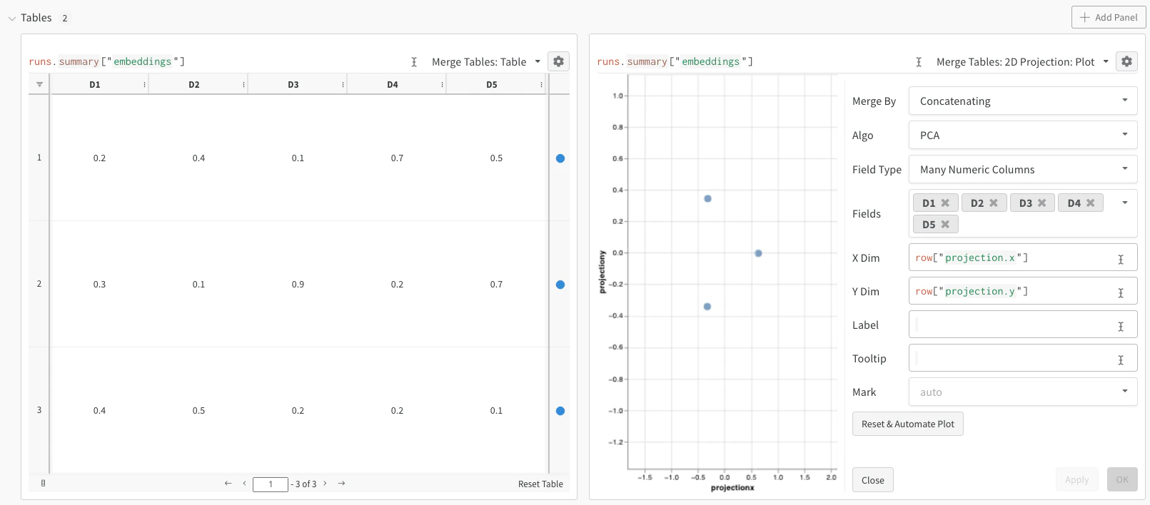
This minimal example shows the smallest amount of code needed to log embeddings and view them in the projector. W&B lets you log embeddings using the wandb.Table class. Consider the following example of three embeddings, each consisting of five dimensions:

import wandb

with wandb.init(project="embedding_tutorial") as run:
  embeddings = [
      # D1   D2   D3   D4   D5
      [0.2, 0.4, 0.1, 0.7, 0.5],  # embedding 1
      [0.3, 0.1, 0.9, 0.2, 0.7],  # embedding 2
      [0.4, 0.5, 0.2, 0.2, 0.1],  # embedding 3
  ]
  run.log(
      {"embeddings": wandb.Table(columns=["D1", "D2", "D3", "D4", "D5"], data=embeddings)}
  )
  run.finish()

After you run the preceding code, the W&B dashboard contains a new Table with your data. Select 2D Projection from the upper-right panel selector to plot the embeddings in two dimensions. W&B automatically selects smart defaults, which you can override in the configuration menu by clicking the gear icon. In this example, W&B uses all five available numeric dimensions.

Digits MNIST

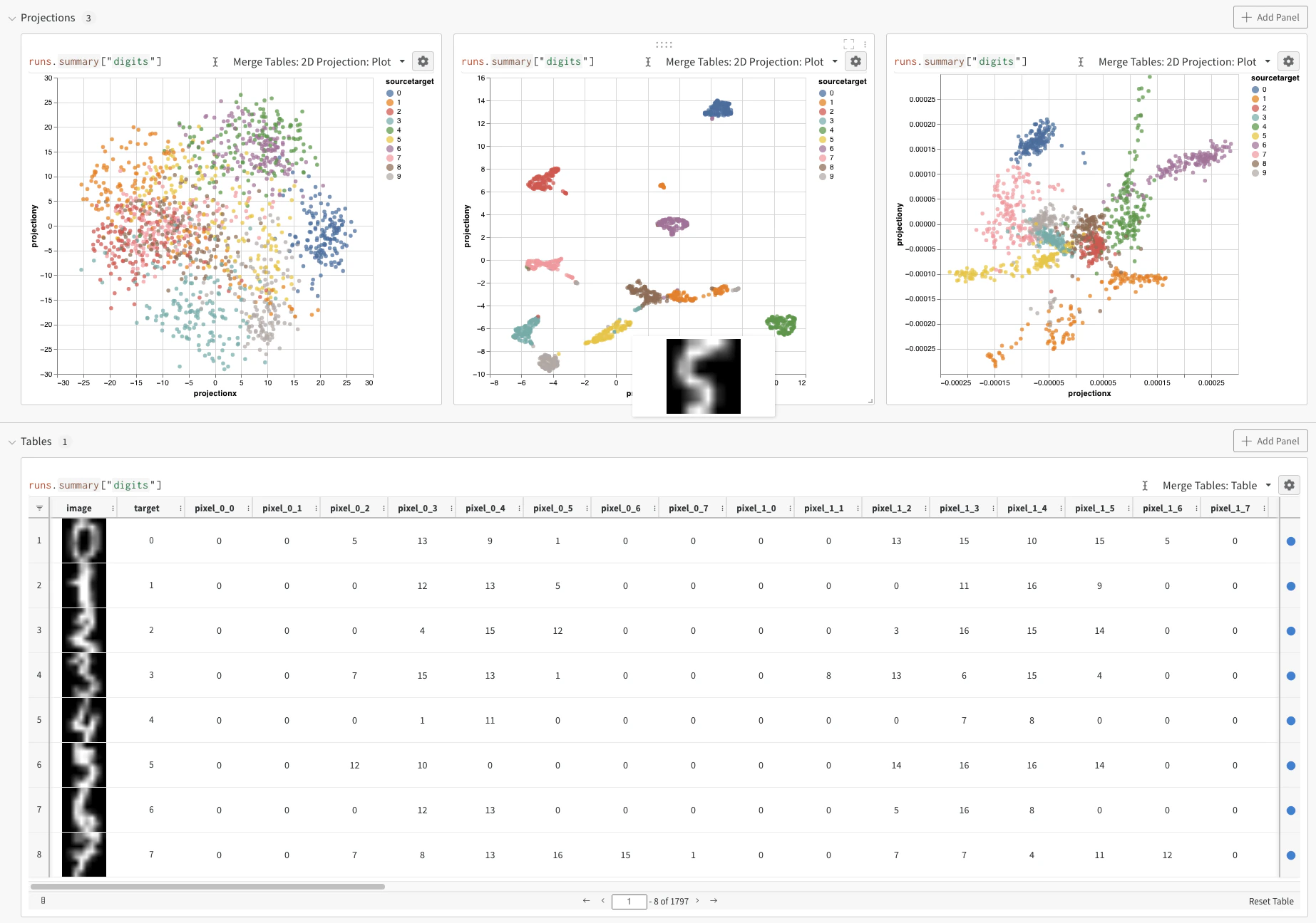
The next example demonstrates a more realistic workflow with higher-dimensional data and richer overlays. While the preceding example shows the basic mechanics of logging embeddings, you typically work with many more dimensions and samples. Consider the MNIST Digits dataset (UCI ML hand-written digits dataset) made available through SciKit-Learn. This dataset has 1,797 records, each with 64 dimensions. The problem is a 10-class classification use case. You can also convert the input data to an image for visualization.

import wandb
from sklearn.datasets import load_digits

with wandb.init(project="embedding_tutorial") as run:

  # Load the dataset
  ds = load_digits(as_frame=True)
  df = ds.data

  # Create a "target" column
  df["target"] = ds.target.astype(str)
  cols = df.columns.tolist()
  df = df[cols[-1:] + cols[:-1]]

  # Create an "image" column
  df["image"] = df.apply(
      lambda row: wandb.Image(row[1:].values.reshape(8, 8) / 16.0), axis=1
  )
  cols = df.columns.tolist()
  df = df[cols[-1:] + cols[:-1]]

  run.log({"digits": df})

After you run the preceding code, the UI again presents a Table. Select 2D Projection to configure the embedding definition, coloring, algorithm (PCA, UMAP, t-SNE), algorithm parameters, and overlay. In this case, W&B shows the image when you hover over a point. These are all smart defaults, and you should see something similar with a single click of 2D Projection. Interact with this embedding tutorial example.

Logging options

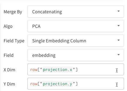
The following sections describe the supported ways to structure embedding data when you log it to W&B. You can log embeddings in several formats:

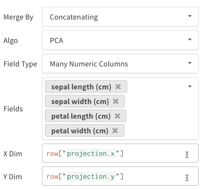
• Single embedding column: Often your data is already in a matrix-like format. In this case, you can create a single embedding column, where the data type of the cell values can be list[int], list[float], or np.ndarray.
• Multiple numeric columns: The preceding two examples use this approach and create a column for each dimension. W&B accepts Python int or float for the cells.

Just like all tables, you have several options for how to construct the table:

• Directly from a dataframe using wandb.Table(dataframe=df).
• Directly from a list of data using wandb.Table(data=[...], columns=[...]).
• Build the table incrementally row by row (great if you have a loop in your code). Add rows to your table using table.add_data(...).
• Add an embedding column to your table (great if you have a list of predictions in the form of embeddings): table.add_col("col_name", ...).
• Add a computed column (great if you have a function or model you want to map over your table): table.add_computed_columns(lambda row, ndx: {"embedding": model.predict(row)}).

Plotting options

After you log your embeddings, you can adjust how they are projected and rendered. After you select 2D Projection, click the gear icon to edit the rendering settings. Besides selecting the intended columns (see preceding sections), you can select an algorithm of interest along with the desired parameters. The following images show the parameters for UMAP and t-SNE.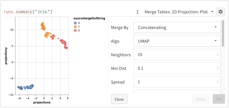

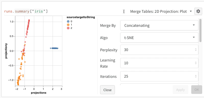
W&B downsamples to a random subset of 1,000 rows and 50 dimensions for all three algorithms.